
When we first onboard a wind farm onto Clir, our software organizes the farm’s raw data into our advanced data model. A series of algorithms are run to enrich and label the data, which is then used to identify, describe and quantify any problems at the farm. Usually, this helps to identify causes of lost energy that were previously unknown or not well understood. We then work with the owner, operator and service provider to resolve or mitigate these losses and any other issues, leading to increased farm production and other benefits.
Occasionally I’ve been asked, “once my wind farm is operating well, how can I continue to leverage Clir?”
I’ll highlight that Clir’s software includes datasets built on industry-leading domain expertise, automated monthly reporting, analysis of wind farm operations, asset health checks, and more, all of which are great reasons to continue using Clir. But specifically, this blog post will focus on wind farm optimization and performance. So, how do our analytics, data sets and machine learning algorithms optimize your wind farm on a recurring basis?
Why recurring analytics are needed
Anecdotally, people in the wind industry understand that at a given wind farm, there’s almost always something going on. High wind turbine availability and performance are achieved through rapid detection and intervention rather than by the turbines operating for months or years reliably in isolation. Wind farm optimization is not permanent. Further, most or all wind farms have intermittent and/or persistent problems.
With the first analysis of a farm, our platform ingests and analyzes millions of data points. This represents a snapshot of the wind farm at that time and any historical issues that were already resolved. Frequently, a wind farm will have been operating for several years before applying our analytics. Almost certainly the wind farm has decades left in its lifetime. What’s going to happen over those decades? What new issues will arise and at what frequency? How often are things actually changing at a turbine or farm?
Our software offers an independent third-party view of any changes made to a turbine or farm which enables us to quickly detect new issues and deliver insights faster than traditional methods. Two of our Machine Learning Engineers, Sam Reh and Shane Butler, have developed a new algorithm that automatically identifies abrupt step-changes in a turbine’s power curve. Each step change's magnitude is quantified based on IEC 61400-12-2: Power performance of electricity producing wind turbines based on nacelle anemometry. Power curve step changes are automatically categorized and prioritized for further investigation based on magnitude, timing and frequency.
Optimization in action
Figure 1 shows an example power curve shift. The shift occurred at wind turbine generator (WTG) X on January 5, 2021, when the power curve abruptly became 14.2% less energetic. Orange dots are before the shift and blue dots are after the shift. This power curve shift was detected by Clir’s machine learning algorithm. Table 1 presents five examples of algorithm output, including the example in Figure 1.
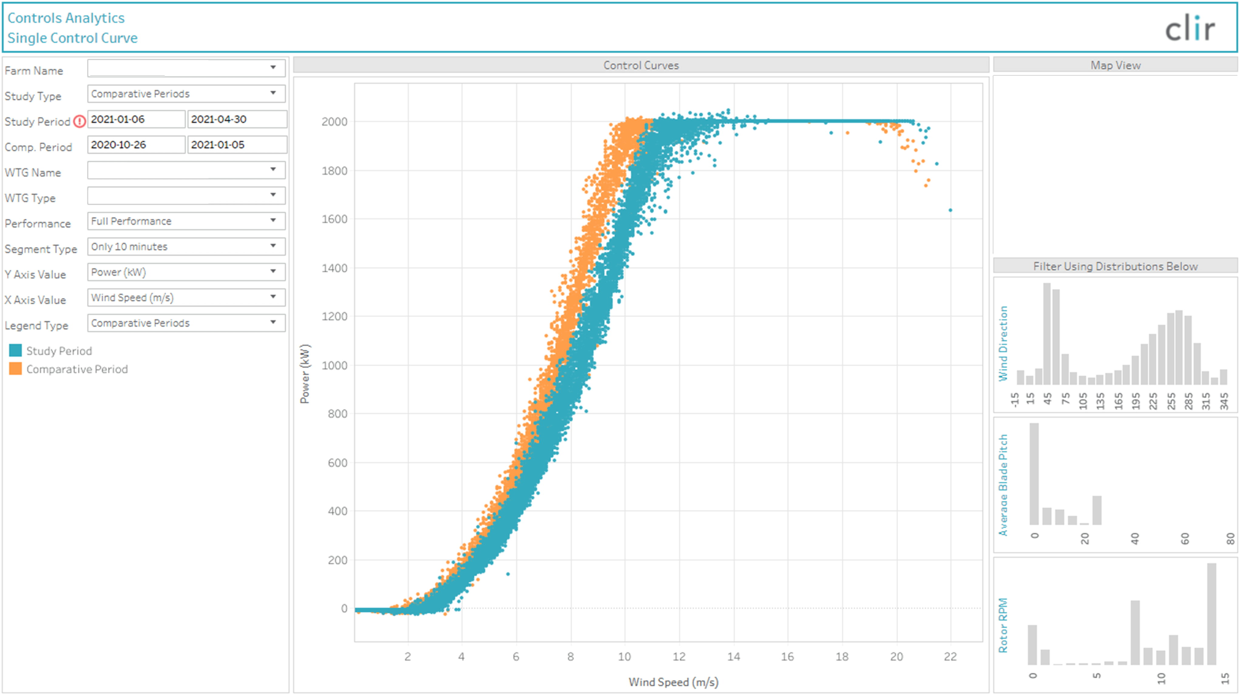
Figure 1: Example power curve shift.
Table 1: Example output from Clir’s power curve change detection algorithm.
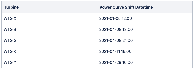
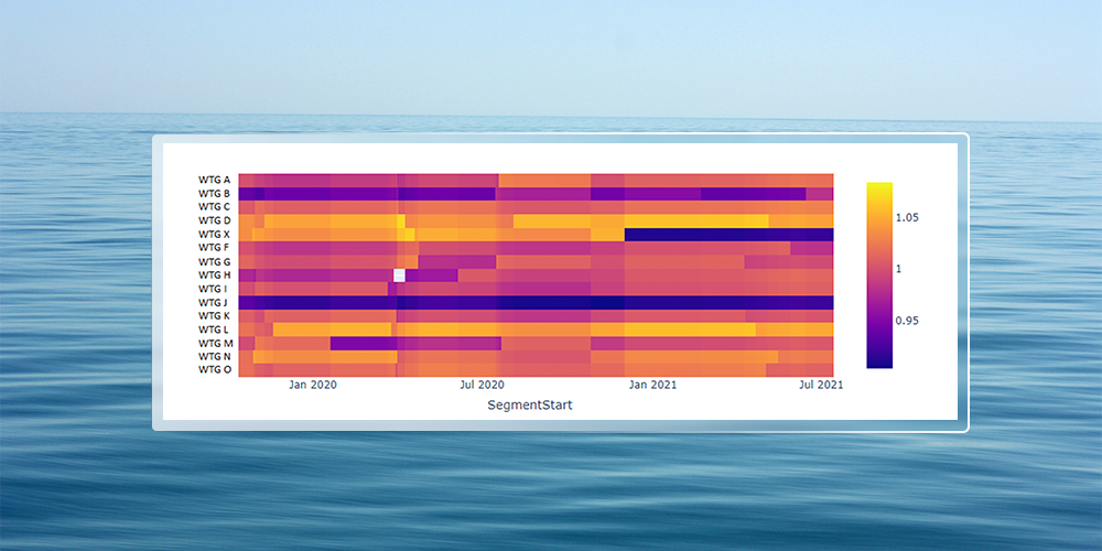
Figure 2 is a heatmap showing quantified power curves over time. Each row represents a turbine, time is on the horizontal axis and power curve changes are indicated by abrupt colour changes. The metric shown in this heatmap is called the Clir Power Curve Benchmark.
The benchmark is calculated at each turbine over time as the ratio of i) the turbine’s annual energy production (AEP), using the analysis methodology from IEC 61400-12-2, to ii) the average turbine AEP at the farm at that time. Essentially, this metric indicates how good the power curve is relative to all other turbines at the farm. For example:
• A value of 1.00 (orange) means the power curve is average.
• A value of 1.10 (yellow) means the power curve is 10% above average.
• A value of 0.90 (blue) means the power curve is 10% below average.
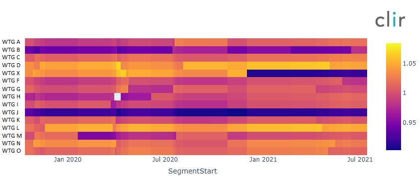
Figure 2: Quantification of power curve changes over time, as measured by the Clir Power Curve Benchmark.
Figure 2 shows benchmark values changing fairly regularly. You might wonder how our algorithm can reliably evaluate performance based on apparently short periods. It only quantifies performance when a sufficient sample size is available, as defined by IEC 61400-12-2. All relevant power curve bins must be filled or else a portion of the heatmap will be null, as can be seen at WTG H for a short period in 2020. When there is a power curve shift at one turbine, the benchmark value at all turbines will change, since the benchmark is defined relative to farm average.
The heatmap in Figure 2 provides transparency and oversight of turbine interventions, farm operations and performance. The changes in the power curve are of main interest. For example:
• Why did the power curve drop at WTG X in January 2021 but not at adjacent WTGs D or F?
• Why did the power curve drop at WTG D in May 2021?
• Why did the power curve drop at WTG B in April 2021 and then rise in June?
What causes power curve changes?
There are many possible causes of power curve changes including:
• A turbine software update.
• Turbine control parameter changes.
• Pitch or yaw system issues.
• Load sensor errors.
• Nacelle wind measurement configuration changes.
• Hardware changes.
• Component replacements.
Clir’s advanced monitoring software provides actionable insight into when these changes occur. This ensures that any new issues at a wind farm, such as inadvertently introduced underperformance, are quickly identified and addressed. Power curve changes may be intentional, such as seasonal tuning of pitch control, or undesirable/unintentional, such as a software update that reverts to old control parameters.
Inflow conditions are also a key determinant in a turbine’s power curve. However, power curve changes due to varying inflow conditions tend to be gradual or intermittent. Clir’s machine learning algorithm is designed to look for persistent and abrupt step changes, so customers are not distracted by simple inflow-condition-induced changes.
As noted above, a nacelle power curve change may be caused by a wind speed measurement configuration change. These are of interest because, depending on the turbine model and vintage, nacelle wind speed may be used by the turbine in a variety of ways, including active turbine control (more common on older turbine models), turbine starts and stops due to curtailment or cut-in/cut-out wind speeds, and site resource reporting.
Power curve changes are a piece of the puzzle, but not the whole story. Once our algorithms detect a significant power curve change, we investigate further using two approaches in parallel:
1. The change is raised with the wind farm operator or turbine service provider to get the 'boots on the ground' feedback. Is there a known issue with the turbine? Can the change be tied to a work order or an intervention? This often yields important information and resolution options.
2. At the same time, the turbine data is further analyzed using automated and manual tools to determine the probable cause. Any findings detected by Clir’s algorithms are shared with the operator to support the resolution of the issue.
Energy production gains
Once the issue is resolved, we typically want to quantify the associated energy production gains. For example, if a problem began at WTG A on July 6, was identified by Clir on July 11, and was resolved by the operator on August 6, what is the production gain? How much production was lost due to the issue?
• In this example the issue only persisted for one month, which is fairly short, meaning the loss in MWh was relatively small.
• On the other hand, if Clir’s software was not monitoring the farm, then the issue may have persisted unknown for many months or even years, making the loss (and potential gain on an annual basis) larger.
Based on Clir’s experience with a wide variety of wind farm operators and turbine service providers, we generally assume the issue would have persisted for six months to a year before being addressed. This assumption may be conservative or aggressive, depending on the parties and stakeholders involved.
How does your farm compare against others?
Clir also carries out cross-farm benchmarking using diverse datasets across projects, OEMs and service providers. This helps owners understand how the frequency of power curve changes at their farm compares to other farms. This provides insight into how often issues arise at your farm, how often interventions occur, and which farms (or turbines) are problematic, as may be indicated by a high frequency of changes.
The results from an example benchmarking analysis are shown here. The majority of Clir’s clients have opted into this type of voluntary anonymous benchmarking to gain insight into how their farms and fleets compare to others in various regards. The Reference Data Set used here is a subset of the farms on Clir, comprised of more than:
• 100 farms;
• 3000 turbines;
• 8 GW of capacity;
• 10 turbine manufacturers; and,
• 15 countries.
Figure 3 shows the distribution of the number of power curve changes per turbine per year, by farm. Blue indicates the Reference Data Set while red indicates the farm of interest, which is the farm from Figures 1 and 2.
On average, there are 1.4 power curve shifts per turbine, per year. This means that if you have a wind farm with 25 turbines, and power curves are changing at the average rate, there will be around three power curve shifts per month. At any given farm, the rate of power curve changes will vary, as seen in the distribution in Figure 3.
The farm of interest has experienced an average of 1.76 power curve changes per turbine per year, which is above the average of the distribution. The Reference Data Set can be further broken down by turbine manufacturer, service provider, region or any other factors of interest. Our technology continually re-analyzes the benchmarking data as the sample size increases to provide better insights over time.

Figure 3: Distribution of the number of power curve changes per turbine per year, by farm, with the reference data set (blue) and the farm of interest (red).
Figure 4 shows the distribution of the number of days between power curve changes considering all power curve changes in the data set. To put it another way, we can define a constant power curve period as the period between two changes at the same turbine. Figure 4 shows the distribution of constant power curve periods. Again, blue is the reference data set and red is the farm of interest. Figure 5 shows the same thing as Figure 4 but with the reference data (blue) removed so that the farm of interest’s distribution can be seen easier.
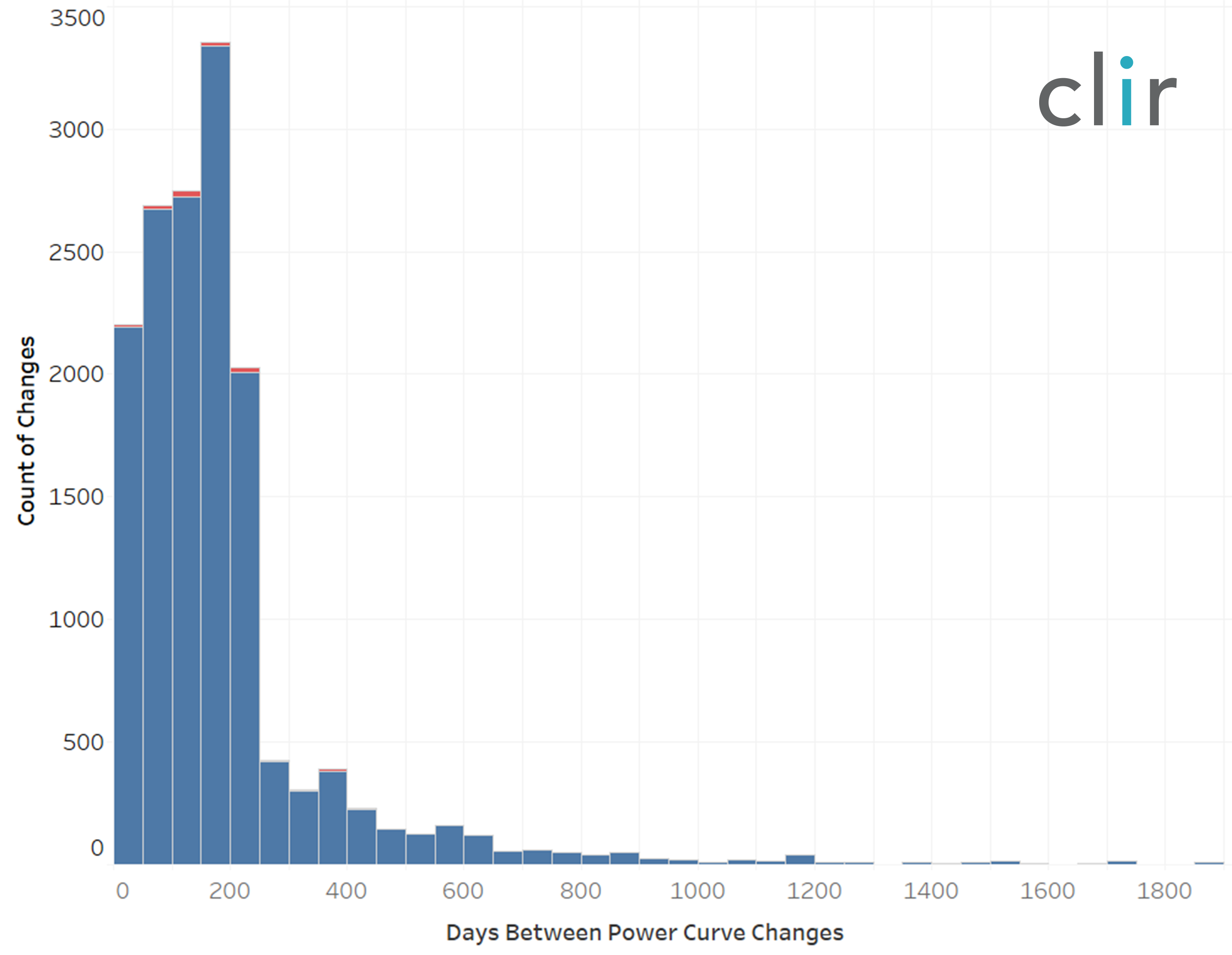
Figure 4: Distribution of the number of days between power curve changes at a turbine, with the reference data set (blue) and the farm of interest (red).
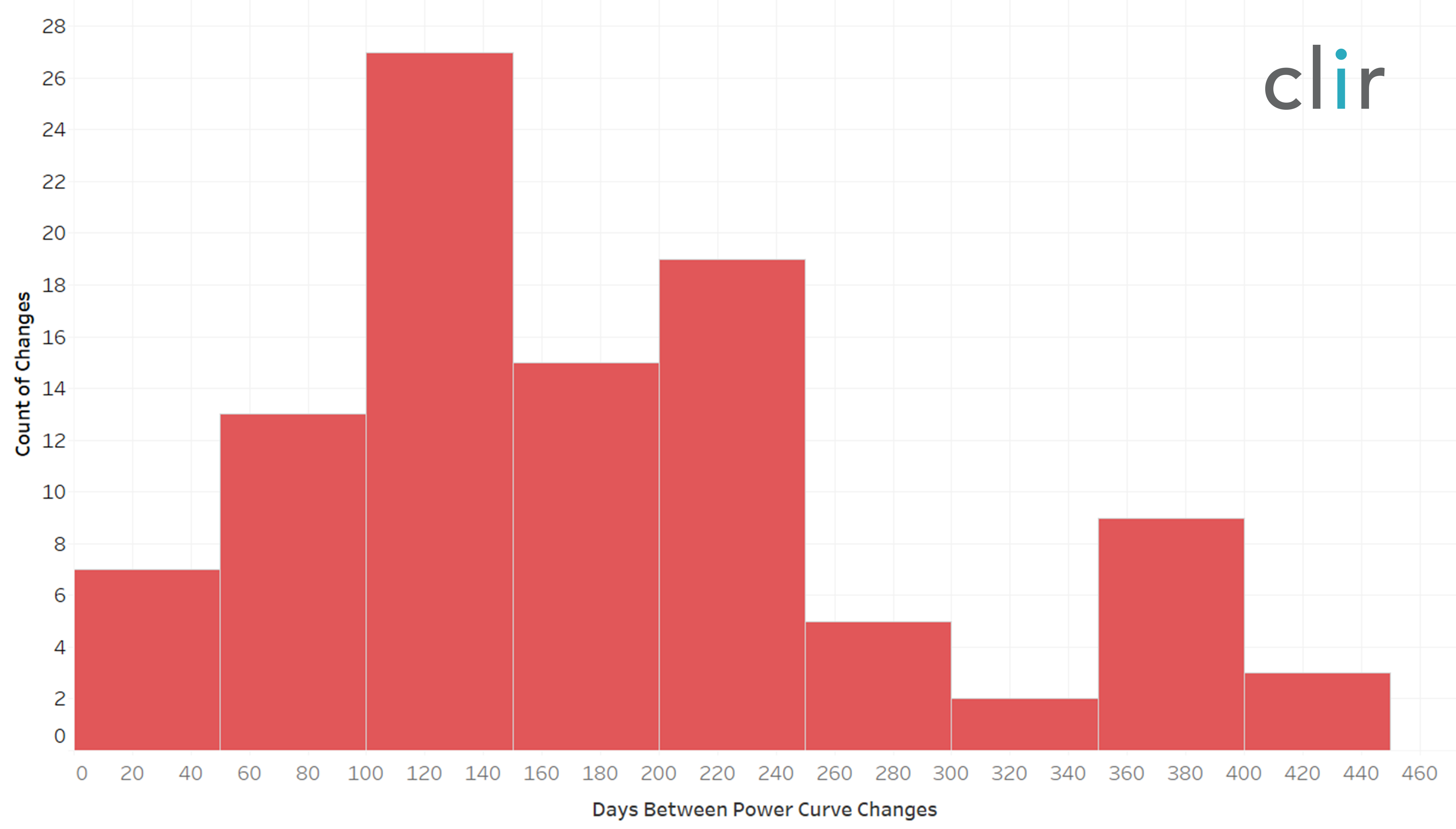
Figure 5: Distribution of the number of days between power curve changes at each turbine, farm of interest (red) only.
The need for continued optimization
At a given wind farm, there’s almost always more going on than is revealed on a typical dashboard. High wind turbine availability and performance are achieved through rapid detection and intervention rather than by the turbines operating for months or years reliably in isolation.
The analysis of a data set comprising 100+ farms and 3000+ turbines reveals an average of 1.4 power curve shifts per turbine per year. Wind farm optimization is not permanent.
Clir’s software offers an independent view of any changes made to a turbine or farm which enables us to quickly detect new issues and deliver insights faster than traditional methods. Optimization of a wind farm can occur on a recurring basis through advanced monitoring that uses machine learning for power curve change detection. The magnitude of each step change is quantified based on IEC 61400-12-2: Power performance of electricity producing wind turbines based on nacelle anemometry. Once a significant power curve change is flagged, Clir investigates further through i) analytics and ii) direct communication with the boots on the ground.
Clir technology provides cross-farm benchmarking to help owners understand how the farm’s frequency of power curve changes compares to other farms. With diverse datasets across projects, OEMs and service providers, it enables insights into how often issues arise at your wind farm, how often interventions occur, and which farms or turbines are persistently problematic, as may be indicated by a high frequency of power curve changes.